Utility

• Patients and clinicians can use this prediction server to classify obstructive and non-obstructive diseases.
• The machine learning (ML) models used in this server were trained on spirometry data of patients. It not only provides an ouput class label but also gives a probability of the prediction.
• Users need to provide only 12 input features for the prediction task.
• Being a non-invasive test, spirometry features can be easily obtained for patients of all age groups, especially children.

Dataset

The dataset contained spirometry investigation reports of 1314 patients from Institute of Pulmocare and Research (IPCR), Kolkata diagnosed with obstructive and non-obstructive diseases. The patients were divided in 2 groups - Group A and Group B consisting of 1163 and 151 patients respectively. The reports of the patients diagnosed with obstructive diseases were labelled as positive and those with non-obstructive diseases were labelled as negative. The reports in Group A were used for training and testing with cross validation (CV-dataset), and the reports in Group B were used as blind dataset. A summary of the dataset is given in Table - 1.

Table - 1: Summary of patient groups in the dataset.

	Group A	Group B
	Used for training and testing with 5-fold cross validation	Used as blind dataset for validation
Patient count	1163	151
Total number of spirometry reports	1172	154
Number of obstructive spirometry reports	1006	103
Number of non-obstructive spirometry reports	166	51

Attributes of spirometry

In spirometry, patients are asked to take a maximal inspiration and, then, expel the air forcefully as quickly as possible into a mouthpiece. The test is repeated following the administration of a bronchodilator. The pre and post bronchodilator values of the following three metrics were used as input:

• Forced Vital Capacity (FVC): It is the volume of air exhaled forcefully and quickly after full inhalation.
• Forced Expiratory Volume in one second (FEV1): It is the volume of air expired during the first second of performing the FVC test.
• Forced Expiratory Flow (FEF25-75): It is the flow (or speed) of air coming out of the lung during the middle portion of a forced expiration. It is measured by taking the mean of the flow during the interval 25-75% of FVC.

For each of the above tests, there are 4 attributes. Thus, there are a total of 12 attributes.

• Pre-bronchodilator (Pre-BD) Value: It is the value of the corresponding metric tested before the administration of bronchodilator.
• Pre-BD Predicted Ratio: It is the percent ratio of pre-bronchodilator (pre-BD) value to the predicted value. There is no normal range of values for the observed metric that is applicable to all individuals in a population. Instead, comparison is made with an expected value for a patient of a particular gender, age and physical characteristics. These are called the predicted values.
• Post-bronchodilator (Post-BD) Value: It is the value of the corresponding metric tested after the administration of bronchodilator.
• Post-BD Predicted Ratio: It is the percent ratio of post-bronchodilator (post-BD) value to the predicted value.

Prediction methodology

Supervised machine learning models were developed for the classification task using Support Vector Machine (SVM), Random Forest (RF), Naive Bayes (NB) and Multi-layer Perceptron (MLP) algorithms. Different performance metrics, such as accuracy, sensitivity, specificity, F1-score, Matthews correlation coefficient (MCC) and area under receiver operator characteristic curve (AUROC) were computed and compared. The optimal model was chosen on the basis of the highest MCC value.

The training dataset used for cross validation was highly imbalanced where the positive to negative ratio (P:N) was 6:1. To handle this imbalance, an undersampling method was used in which the majority (positive) class samples were randomly divided into six disjoint (and, exhaustive) subsets. Then the minority (negative) class samples were concatenated with each positive class subset to obtain six undersampled datasets with P:N = 1:1. Six models were trained with each undersampled dataset and the performance metrics were averaged.

The tuning of hyperparameters was performed for each ML algorithm to improve the performance of the models using grid search technique, which is an exhaustive search using a parameter grid created by taking the cartesian product of pre-specified sets of values for each hyperparameter. Hyperparameter optimization was performed separately for both sets of models - one trained with the whole training set and another with the undersampled datasets. The optimal model wass saved and used in this prediction server.

Performance

Table - 2: Performance of models with 5-fold cross validation

Dataset	Model	Accuracy	Sensitivity	Specificity	F1-score	MCC
Whole training dataset	Support Vector Machine (SVM)	0.835	0.837	0.826	0.897	0.532
	Random Forest (RF)	0.906	0.955	0.609	0.946	0.597
	Naive Bayes (NB)	0.870	0.915	0.602	0.924	0.495
	Multi-layer Perceptron (MLP)	0.918	0.966	0.626	0.953	0.645
Under-sampled datasets	Support Vector Machine (SVM)	0.823	0.825	0.821	0.824	0.650
	Random Forest (RF)	0.822	0.832	0.811	0.824	0.647
	Naive Bayes (NB)	0.800	0.864	0.737	0.813	0.607
	Multi-layer Perceptron (MLP)	0.837	0.853	0.822	0.841	0.682

The MLP model trained with the under-sampled datsets showed optimal performance with MCC of 0.68 and accuracy of 83.7% (Table - 2). This model is used in this prediction server. The hyperparameters chosen by the grid-search algorithm for this MLP model used two hidden layer architecture - 100 nodes in the first hidden layer followed by 100 nodes in the second. The input and output layers used 12 and 1 nodes respectively. An "adam" weight optimizer and a rectified linear unit (ReLU) activation function with constant learning rate of 0.001 was used. The ROC plot of the different models are given in Figure - 1. The performance of the models on blind dataset (Group - B) is given in Table - 3.

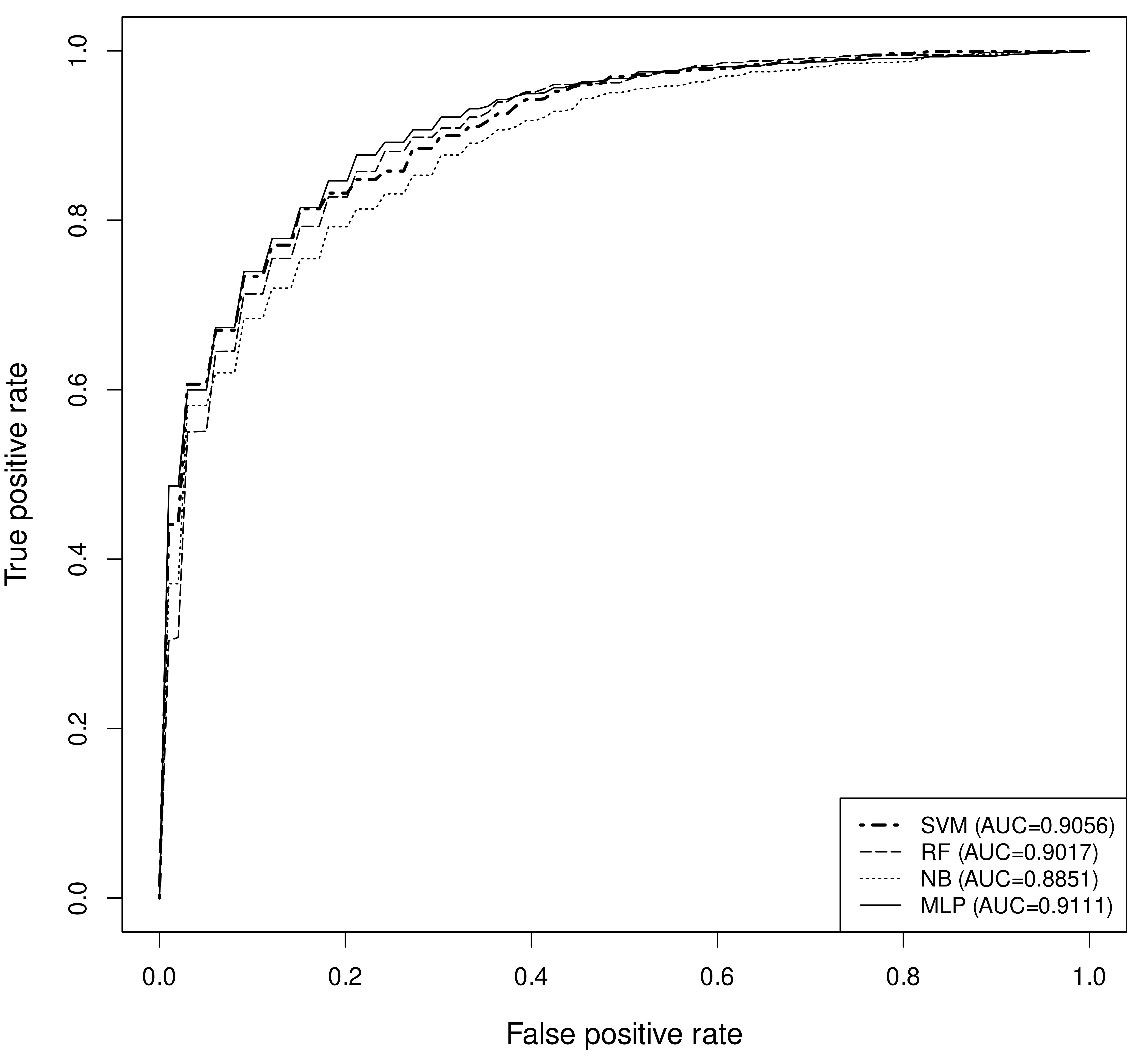
Figure - 1: Receiver Operator Characteristic (ROC) plot of different models. (σ-standard deviation)

Table - 3: Performance of models on predicting the validation dataset

Training Dataset	Model	Accuracy	Sensitivity	Specificity	F1-score	MCC
Whole training dataset	Support Vector Machine (SVM)	0.853	0.897	0.765	0.891	0.667
	Random Forest (RF)	0.835	0.971	0.561	0.887	0.619
	Naive Bayes (NB)	0.823	0.944	0.580	0.877	0.586
	Multi-layer Perceptron (MLP)	0.857	0.986	0.596	0.902	0.677
Under-sampled datasets	Support Vector Machine (SVM)	0.854	0.898	0.766	0.892	0.669
	Random Forest (RF)	0.862	0.902	0.781	0.897	0.687
	Naive Bayes (NB)	0.855	0.926	0.712	0.895	0.665
	Multi-layer Perceptron (MLP)	0.849	0.886	0.774	0.887	0.663