MDPD website navigation map
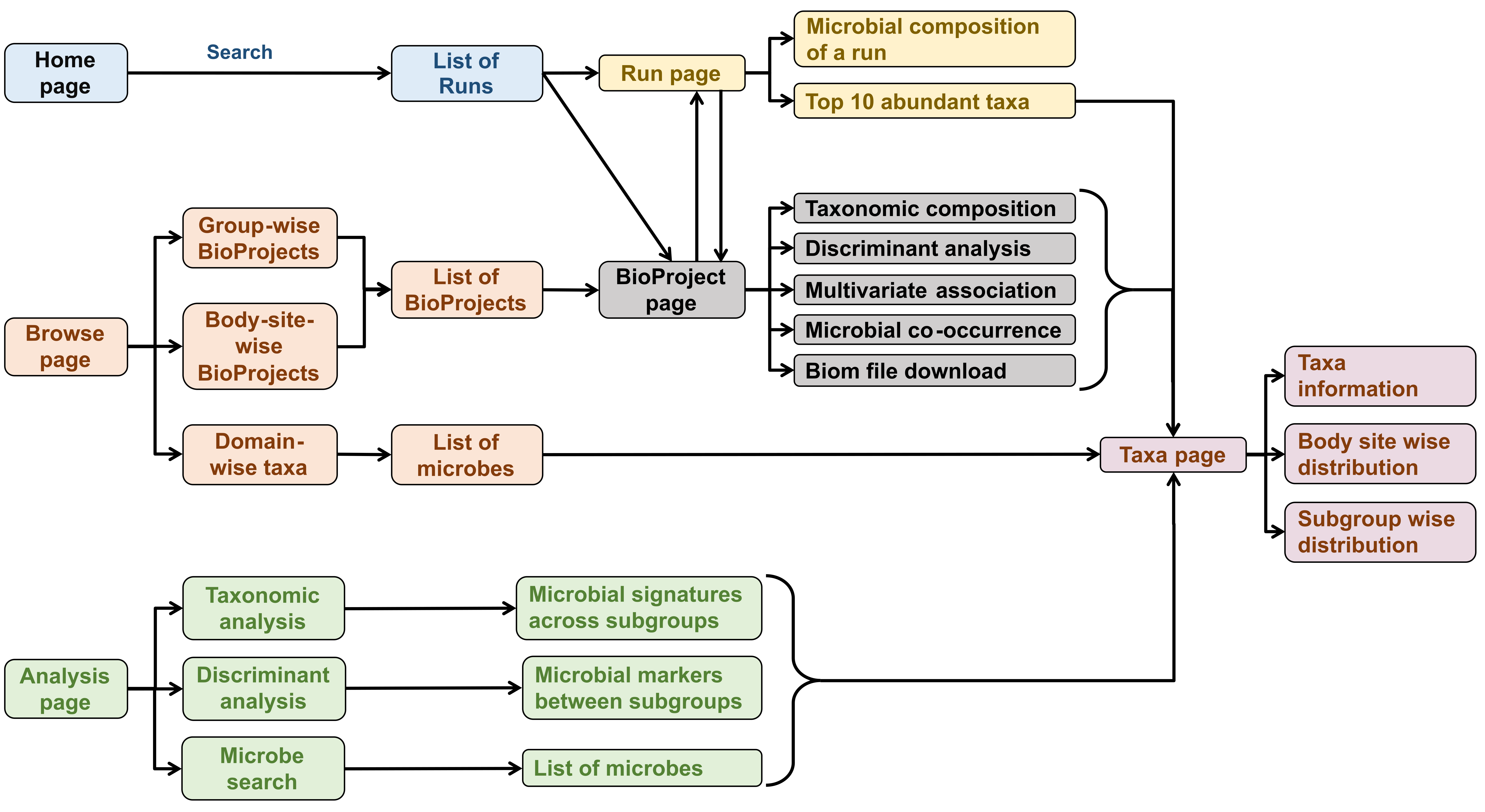
Home page
The home page provides a brief introduction of MDPD and a Search option.
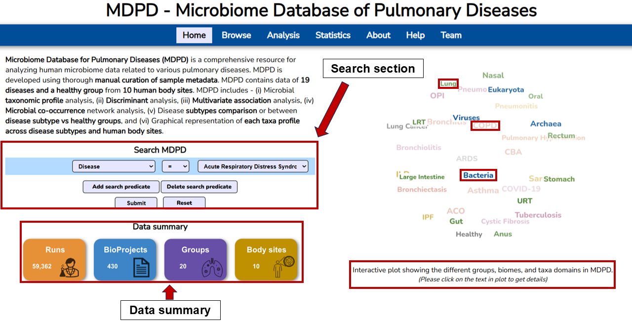
Search MDPD
MDPD is equipped with a "Search Section" that allows users to generate extensive and customizable queries with just a few clicks. Users can search runs/samples using relevant technical metadata, including Group (diseases, healthy), Assay type (Amplicon-16S, Amplicon-ITS, WMS), Body site (Lung, Gut), Library layout (Single, Paired), Country, and Year.
For example, the screenshot below shows a user query to search for runs/samples that were from COPD individuals, sequenced by Amplicon-16S, and obtained from the Lower Respiratory Tract.
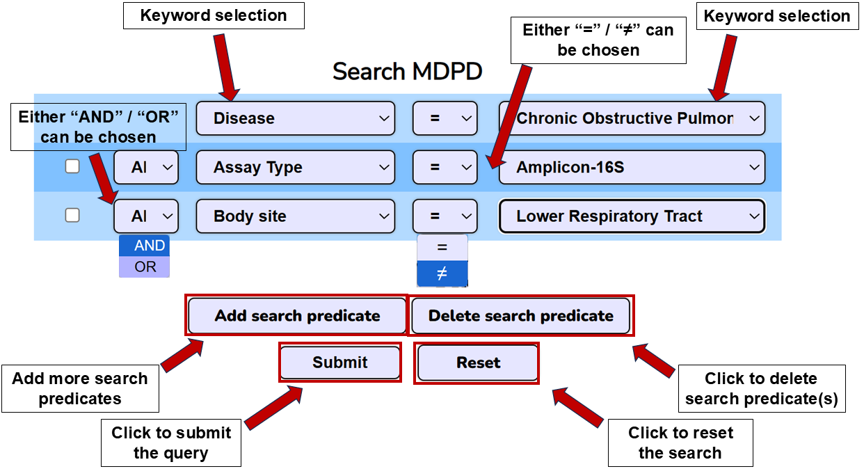
Users can also make some complex inquiries.
- Choose
=/≠/</>/<=/>=for predicates, and chooseAND/ORto combine predicates. - Add or delete search predicates.
- Reset all the search predicates.
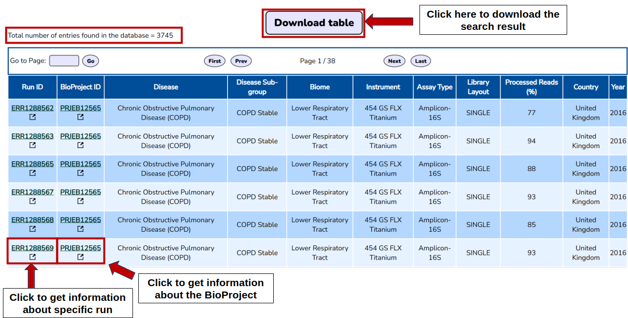
Result of search queries
Search result page provides information of the runs matching the input query in a tabular format. It contains different attributes - Run ID, BioProject ID, SRA Study ID, Disease, Disease Subgroup, Body site, Instrument, Assay Type, Library Layout, Processed reads (%), Country, and Year. The table displayed in the search result can be downloaded in CSV format by clicking on the "Download table" button located at the top of the page. An example search result is shown below.
- Click on each Run ID to view the details of the run in the Run page.
- Click on BioProject ID to view the details of the BioProject in the BioProject page.
Browse page
The browse page can be accessed from the menubar present at the top of every page. It has three sections to find the BioProjects and the microbes.

Group-wise BioProjects
This allows users to browse BioProjects on the basis of the 19 pulmonary diseases (categorized into five classes) and the healthy group.
- Obstructive - Asthma, Asthma-COPD Overlap (ACO), Bronchiectasis, Bronchitis, COPD and COPD- Bronchiectasis Association (CBA).
- Restrictive – Acute Respiratory Distress Syndrome (ARDS), Cystic Fibrosis, Interstitial Lung Disease (ILD), Idiopathic Pulmonary Fibrosis (IPF), Sarcoidosis and Pneumonitis.
- Infectious – Bronchiolitis, COVID-19, Pneumonia, Tuberculosis, Other Pulmonary Infections (OPI).
- Vascular – Pulmonary Hypertension.
- Malignancy – Lung Cancer.
- Healthy – Healthy.
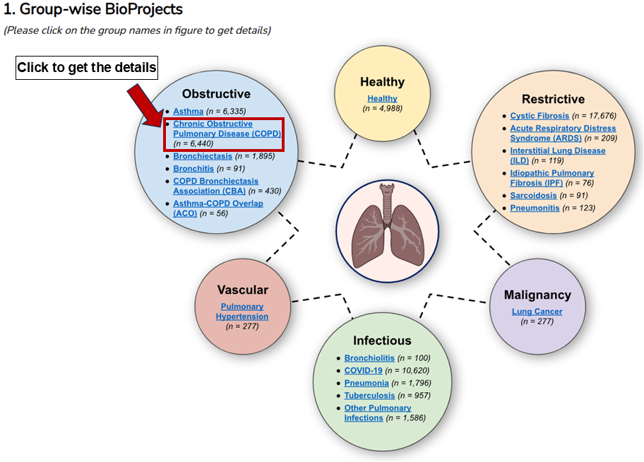
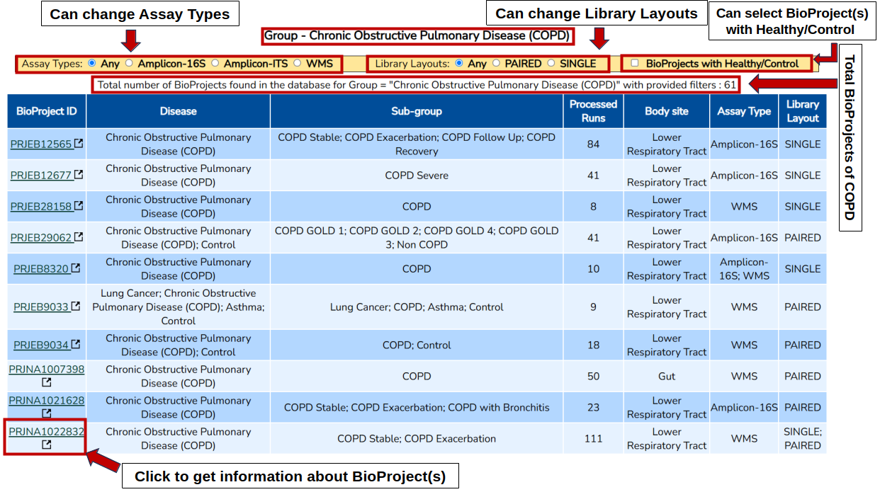
The 'n' represents the number of runs/samples in the respective group. Click on the group names to get the details as shown in the following figure.
- Shows the basic information about the BioProjects in tabular format.
- Click on the BioProject ID to view details in the BioProject page.
- Customize the list using the filter buttons.
Body-site-wise BioProjects
This allows the users to browse BioProjects across the 10 body sites - (i) Nasal, (ii) Oral, (iii) Upper Respiratory Tract, (iv) Lower Respiratory Tract, (v) Lung, (vi) Stomach, (vii) Large Intestine, (viii) Gut, (ix) Rectum and (x) Anus.
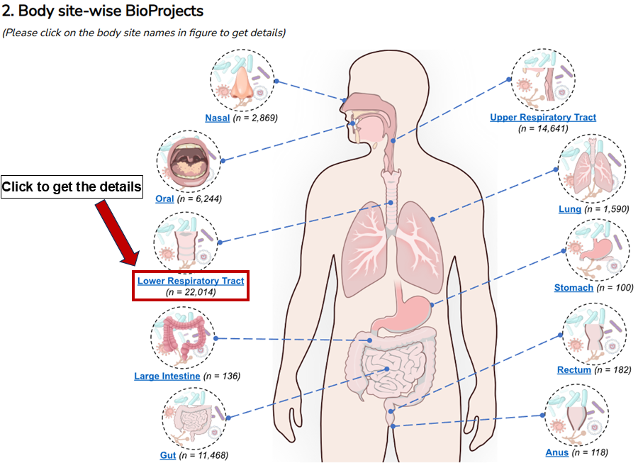
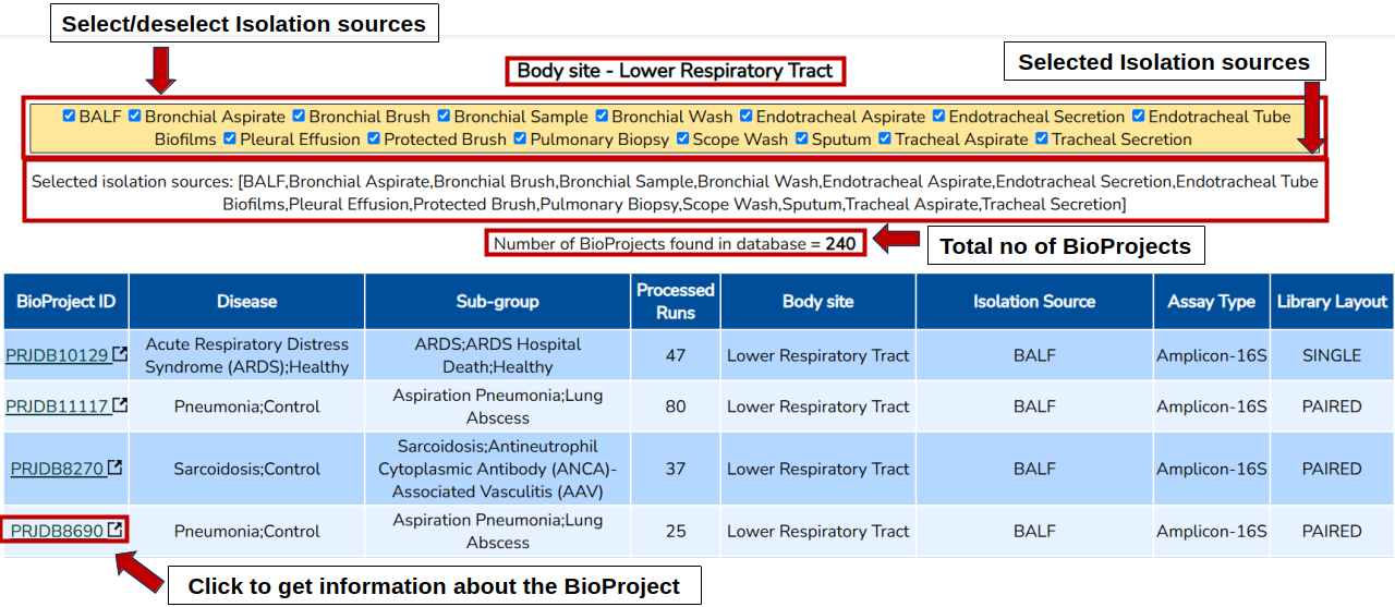
The 'n' represents the number of runs/samples in the respective body site. Click on the body sites to get the details as shown in the following figure.
- Shows the basic information about the BioProjects in tabular format.
- Click on the BioProject ID to view details in the BioProject page.
- Customize the list using the filter buttons.
Domain-wise taxa
This allows the users to browse microbes and their abundances across subgroups and body sites across the four domains - (i) Bacteria, (ii) Viruses, (iii) Eukaryota, and (iv) Archaea.
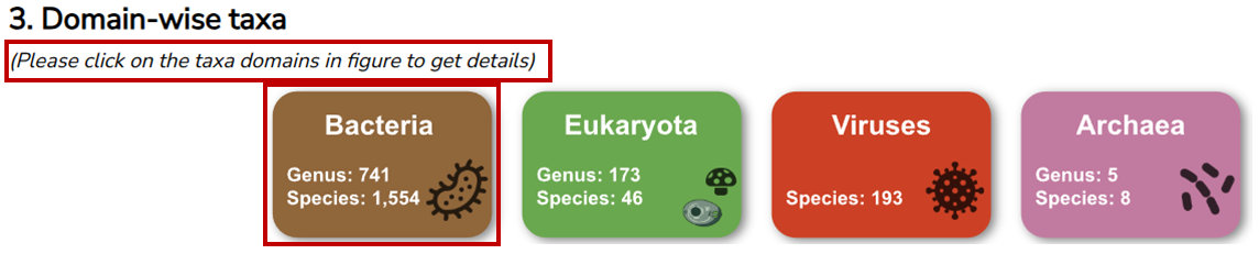
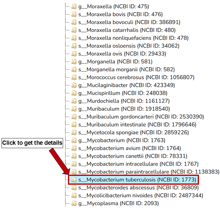
Click on any domain to get a list of microbes as shown in the following figure. Click on the microbe names to view taxa information and their abundances across subgroups and body sites in the Taxa page.
The taxon information were retrieved from "bugphyzz: A harmonized data resource and software for enrichment analysis of microbial physiologies" accessed on 19th January, 2025.
Run page
The Run page provides:
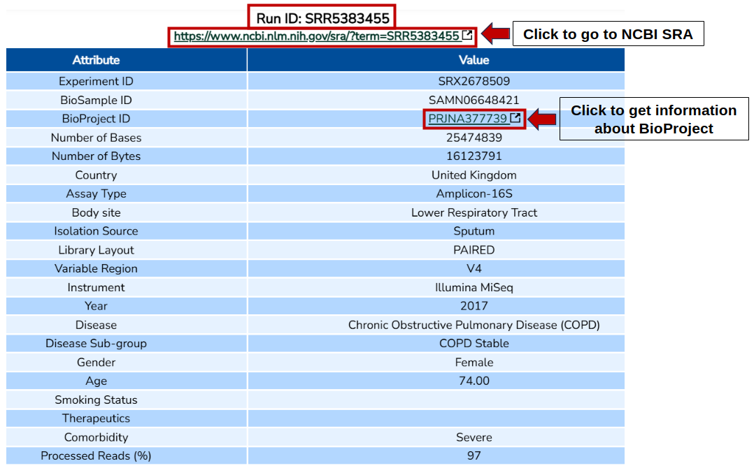
Basic information of a run
It includes different attributes associated with the run/sample - Run ID, Experiment ID, BioSample ID, Number of Bases, Number of Bytes, Country, Assay Type, Body site, Isolation Source, Library Layout, Variable Region, Instrument, Year, Disease, Disease Subgroup, Gender, Age, Smoking Status, Therapeutics, Comorbidity, and Processed Reads (%). A link is available that leads to the NCBI SRA page. Click on the BioProject ID to view the BioProject details in the BioProject page.
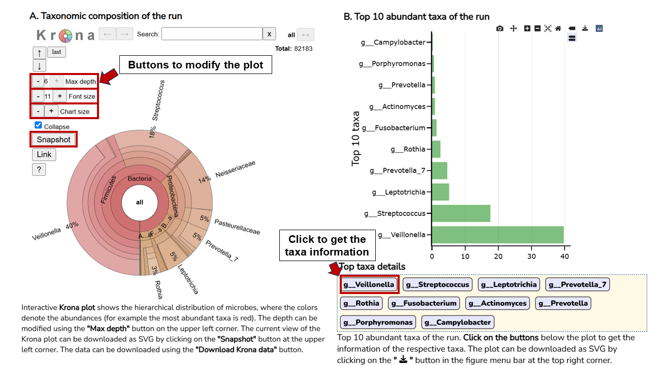
Microbial composition of the run
The microbial composition of the run is visualized as an interactive Krona plot. The colors denote the abundance of the microbes, where red color represents the abundant ones. Interact with the Krona plot using the buttons available in the upper left corner to change the depth, font, and chart size. Click on the "Snapshot" button to download the plot in SVG format.
Top 10 abundant taxa in the run
The top 10 taxa of the run are visualized as a bar plot. Hover on the bar to view the relative abundance value of a particular taxon. Click on "↓" button at the top right corner of the plot to download the Krona plot in SVG format. Click on the microbe buttons below the plot to view detailed information in the Taxa page.
BioProject page
The BioProject page provides:
Basic information of a BioProject
It includes different attributes associated with the BioProject - BioProject ID, SRA ID, Disease subgroup(s), Isolation Source, Body Site, Assay Type, Instrument, Library Layout, Year, Processed Runs, Variable Region, PMID and Country. A link is available that leads to the NCBI BioProject page.
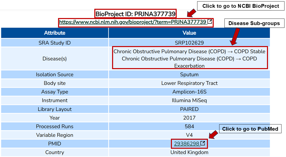
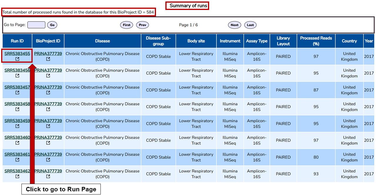
Metadata of runs in the BioProject
BioProject page shows the metadata of available runs in the BioProject. Click on the Run ID to view the details of the run in the Run page.
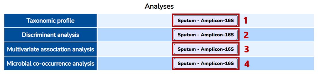
Analyses of runs in the BioProject
Users can perform different types of analyses of runs in the BioProject.
Download .biom file of the BioProject
Users can download the .biom file of the respective BioProject.

Microbial taxonomic profile of runs in a BioProject
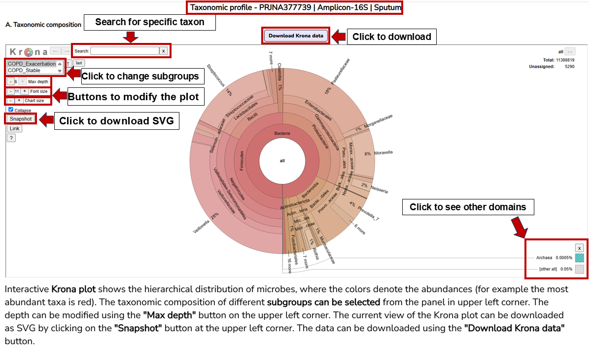
Taxonomic composition
The taxonomic composition of the all runs of each subgroup and isolation sources in the BioProject is visualized as an interactive Krona plot. The hierarchical taxonomic classification can be seen with this plot with genus/species at the outer ring and the inner ring denoting the domains. The color gradient shows the abundance of microbes where red color indicating more abundant taxa. Select the subgroups and modify the krona plot by changing the depth, font, and chart size using the buttons available in the upper left corner. Click on the "Snapshot" button to download the plot in SVG format. Click on the "Download krona data" to download the plot in HTML format.
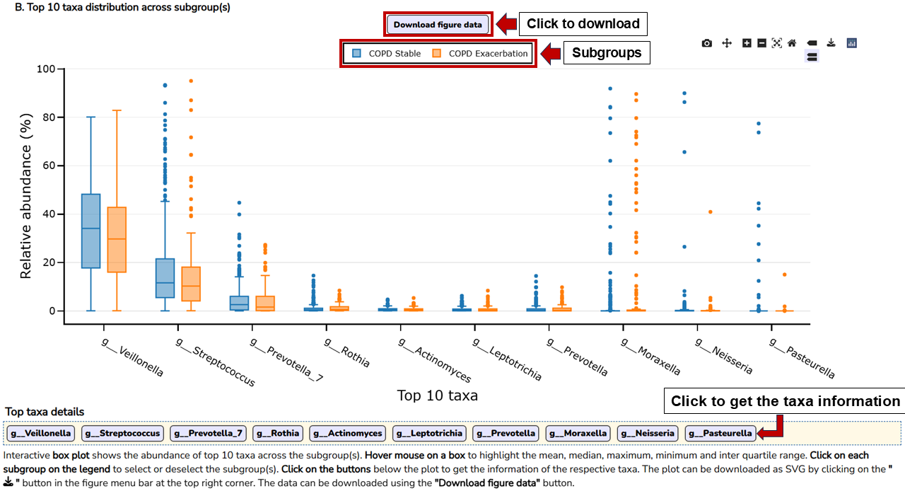
Top 10 abundant taxa in each subgroup of the BioProject
The top 10 abundant taxa in each subgroup of the BioProject are visualized as a box plot. Each box shows the distribution of relative abundance of a microbe across the runs in the BioProject. Hover on a particular box to view the min, median, max values of that taxon. Click on "↓" button at the top right corner of the plot to download the plot in SVG format. Click on "Download figure data" button to download the data used to plot the figure. Click on the microbe buttons below the plot to view detailed information in the Taxa page.
Discriminant analysis of runs in a BioProject
It allows users to find the differential microbial signatures between the subgroups of the BioProject. The differential taxa are visualized as a bar plot. The length of the bar denotes the LDA score (log10) or log2 fold change depending on the chosen method. LDA score signifies the effect size of each differentially abundant microbe. Click on "↓" button at the top right corner of the plot to download the plot in SVG format. Click on "Download figure data" button to download the data used to plot the figure. Click on the microbe buttons below the plot to view detailed information in the Taxa page.
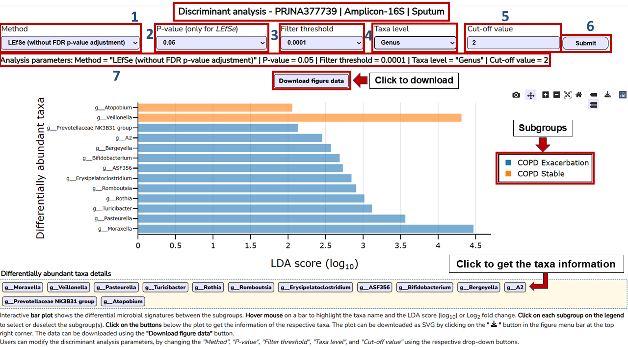
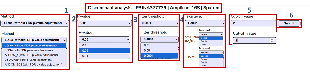
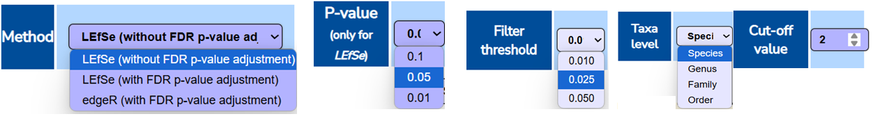
Users can modify different parameters of the analysis:
- Statistical "Method"
- P-Value (Only for LEfSe)
- Filter threshold
- Taxa level (Order through Genus in Amplicon-16S/Amplicon-ITS and Order through species in WMS)
- Cut-off value
Click on the "Submit" button to perform the analysis with the updated parameters. Users can also see the selected parameters for the current analysis.
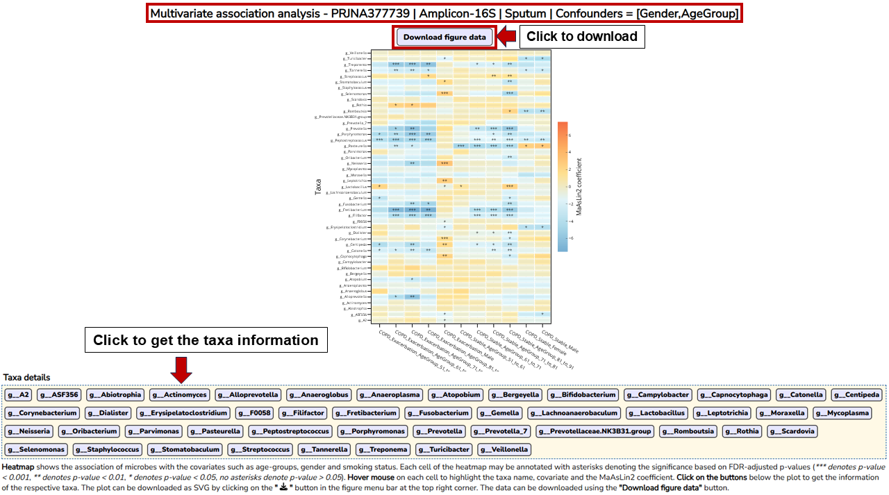
Multivariate association analysis of runs in a BioProject
It allows users to find associations of the microbes with the
covariates such as age groups, gender, and smoking status.
MaAsLin2 is used to find the associations. Each cell of the
heatmap is annotated with asterisks denoting the significance
based on FDR-adjusted p-values (*** denotes
p-value < 0.001, ** denotes
p-value < 0.01, * denotes
p-value < 0.05, no asterisks denote
p-value > 0.05). Positive MaAsLin2 coefficient
indicates a positive correlation between microbe and the covariates
while negative coefficient denotes inverse associations. Hover
mouse on each cell to highlight the taxa name, covariate and
the MaAsLin2 coefficient. Click on "↓" button at the top right
corner of the plot to download the plot in SVG format. Click on
"Download figure data" button to download the data used to plot
the figure. Click on the microbe buttons below the plot to view
detailed information in the
Taxa page.
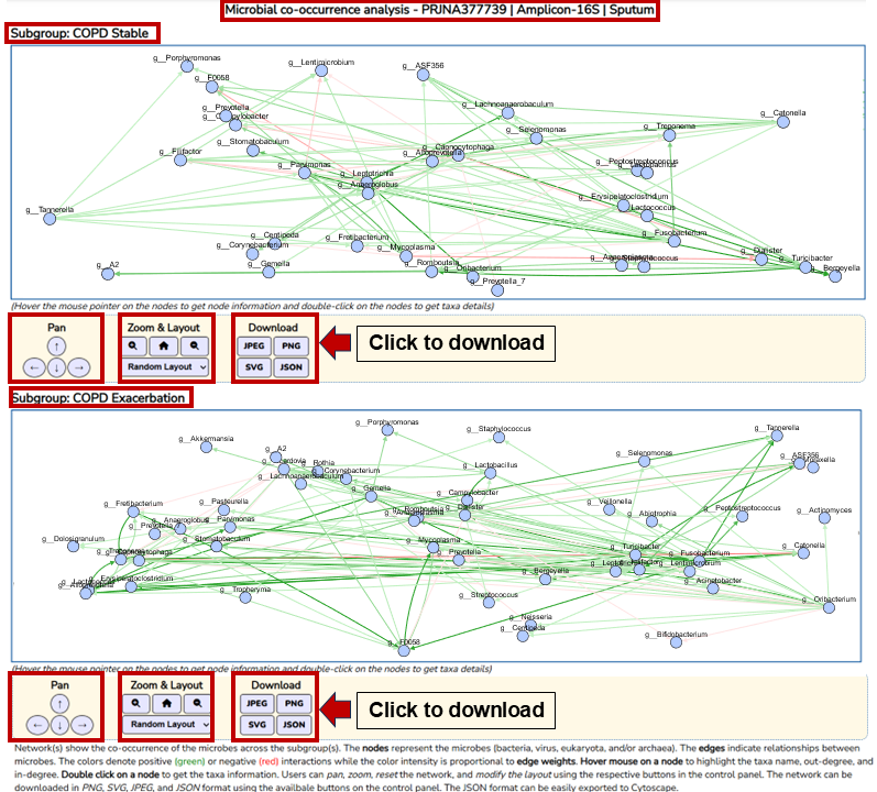
Microbial co-occurrence analysis of runs in a BioProject
It allows the users to visualize the dynamics of microbial community with co-occurrence networks. Gradient Boosted Linear Model (GBLM) method was applied to build the networks. The nodes represent the microbes (bacteria, virus, eukaryota, and/or archaea). The edges indicate relationships between microbes. The colours denote positive (in green) or negative (in red) interactions while the color intensity is proportional to edge weights. Change the layout of network using the drop-down menu. Click on "JPEG", "PNG", "SVG", and "JSON" buttons to download the network in the respective formats. Double click on a node to view detailed information of the taxa in the Taxa page.
Taxa page
Basic information of the taxon
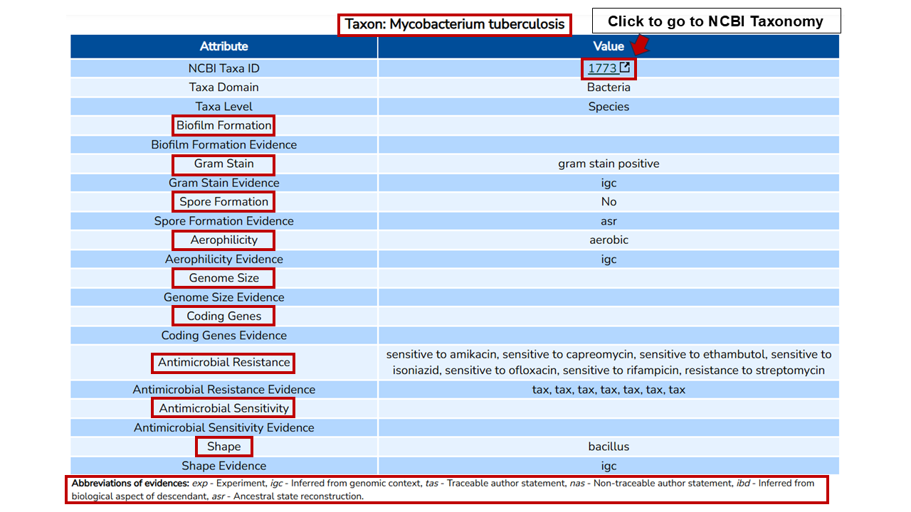
Users get information about (i) Biofilm formation, (ii) Gram staining, (iii) Spore formation, (iv) Aerophilicity, (v) Genome size, (vi) Coding genes, (vii) Antimicrobial resistance, (viii) Antimicrobial sensitivity, (ix) shape, and (x) Pathogenicity.
The abbreviations of the evidences supporting an annotation are as follows:
- EXP: Experiment
- IGC: Inferred from genomic context
- TAS: Traceable author statement
- NAS: Non-traceable author statement
- IBD: Inferred from biological aspect of descendant
- ASR: Ancestral state reconstruction
Relative abundances of the taxon across body sites
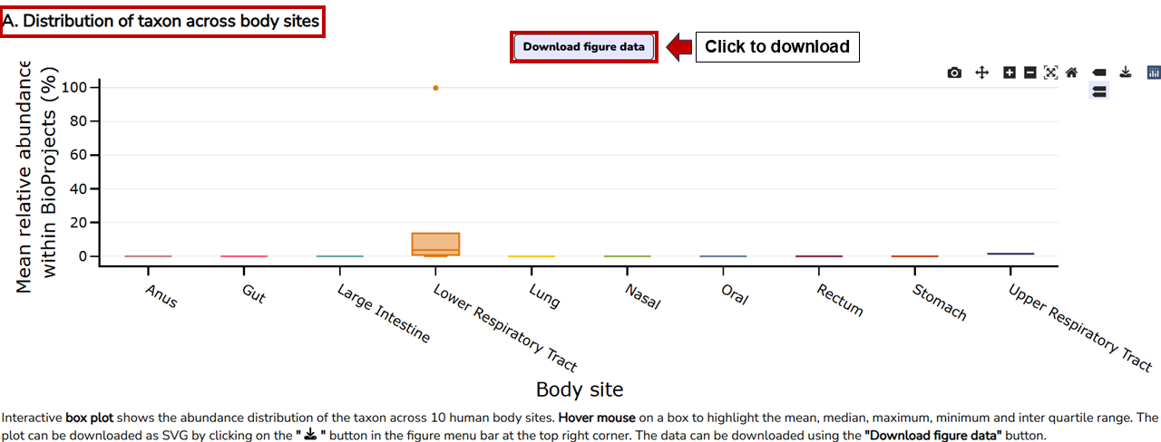
The plot can be downloaded as a SVG image by clicking on the "↓" button in the menu bar located at the top right corner of the plot.
Relative abundances of the taxon across subgroups
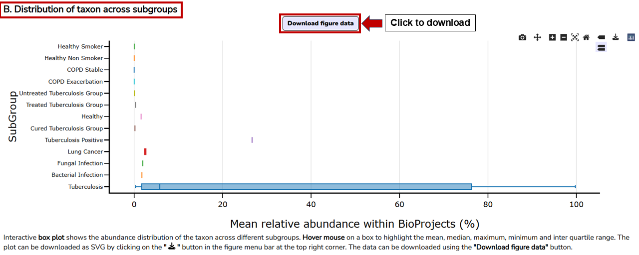
The plot can be downloaded as a SVG image by clicking on the "↓" button in the menu bar located at the top right corner of the plot.
Analysis page
The Analysis page can be accessed from the menubar present at the top of every page. It provides three analyses for user-defined queries. It allows to find the microbial signatures of different subgroups, BioProjects, and isolation sources within a group. It allows to identify microbial markers across different subgroups, BioProjects, and isolation sources of one or more groups. It also allows users to search taxon details.

User-defined taxonomic analysis
It helps researchers to understand if a microbe has the similar trend across subgroups or in BioProjects or different or no trend. For simplicity, the subgroups with highest number of runs/samples were taken for the analysis. However, users can use other subgroups as they can download the .biom files of respective BioProject(s).
Input
Users can select the Groups, which will open a dialog box where they can select/deselect options such as Subgroups, Isolation Source, Assay Type and Library Layouts. For example, Group – Healthy is shown here and the selected parameters are:
- Subgroup – Healthy Smoker and Healthy Non Smoker
- Isolation Source – BALF, Sputum, and Stool
- Assay Type – Amplicon-16S
- Library Layout – PAIRED and SINGLE
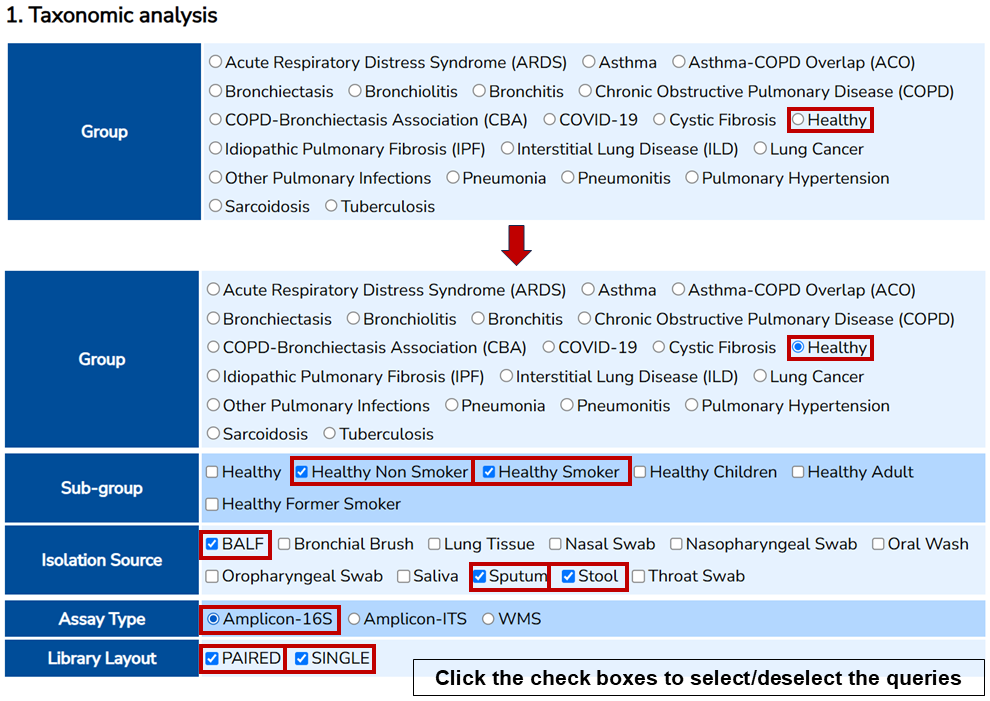
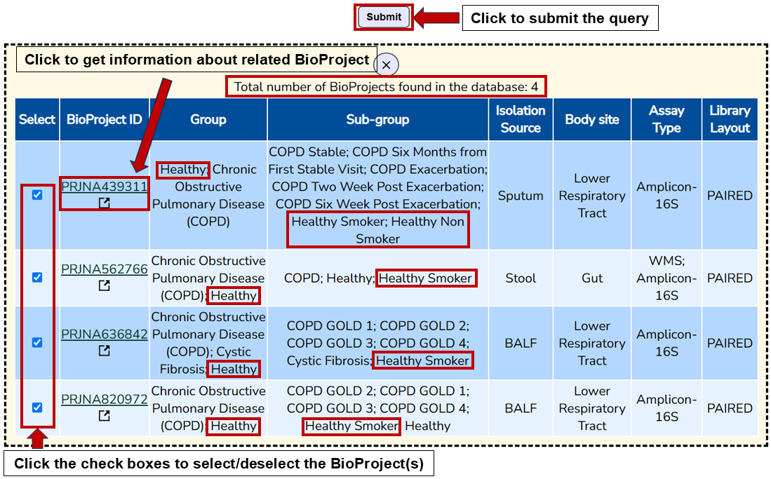
Users can also customize the BioProjects selection. Among the selected BioProjects, only the runs that satisfy the selection criteria above are used for the analysis.
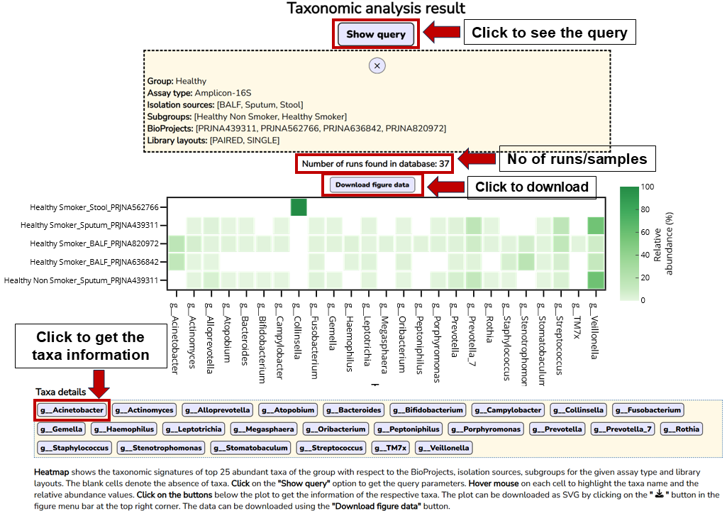
Output
This heatmap shows the relative abundances (%) of the microbes across the queried Subgroups, Isolation Sources, and BioProjects. It shows the top 25 abundant taxa. The blank cells indicate the absence of the taxa. Hover mouse on each cell to highlight the taxa name, subgroup, isolation source, BioProject and the relative abundance. Click on "↓" button at the top right corner of the plot to download the plot in SVG format. Click on "Download figure data" button to download the data used to plot the figure. Click on the microbe buttons below the plot to view detailed information in the Taxa page.
User-defined discriminant analysis
It helps researchers to understand if a microbial marker is unique to a subgroup, or shared by different subgroups. For simplicity, the subgroups with highest number of runs/samples were taken for the comparison. However, users can use other subgroups as they can download the .biom files of respective BioProject(s).
Input
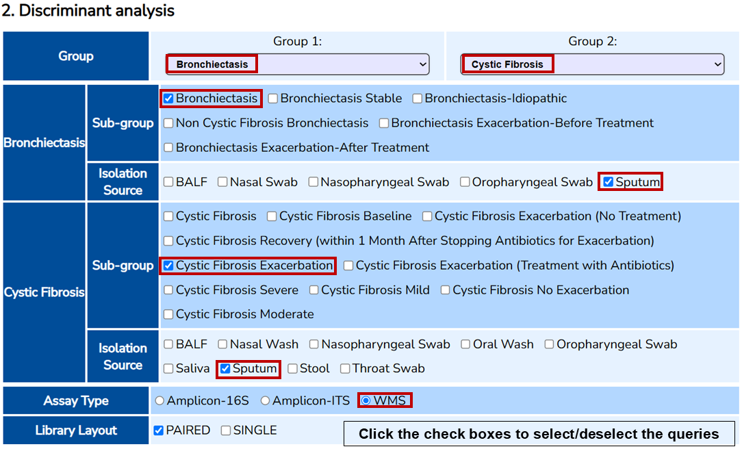
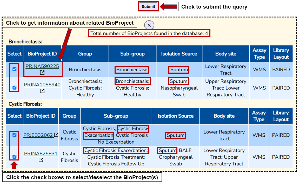
Users can select the Groups (1 and/or 2) to compare. For each selection a dialog box gets opened where they can select the subgroups and isolation sources, and it also allows the selection of assay type and library layouts. For example, comparison between "Bronchiectasis and Cystic Fibrosis" is shown here and the selected parameters are:
- Subgroups – Bronchiectasis and Cystic Fibrosis Exacerbation
- Isolation Source – Sputum
- Assay Type – WMS
- Library Layout – PAIRED

Users have several options to modify the analysis.
- Users can change the statistical "Method"
- Users can set different "P-Value" (Only for LEfSe)
- Users can set different "Filter threshold"
- Users can change the "Taxa level"
- Users can modify the "Cut-off value"
- Click to "Submit"
Users can also customize the BioProjects selection. Among the selected BioProjects, only the runs that satisfy the selection criteria above are used for the analysis.
Output
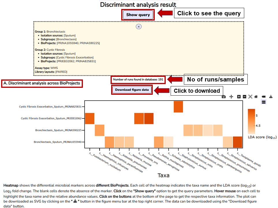
Individual BioProject wise
This heatmap shows the microbial markers in individual BioProjects of the respective subgroups. Here, LEfSe method was chosen to find the differential markers. The blank cells indicate absence of the taxa. The colour intensity denotes the LDA score (log10). LDA score signifies the effect size of each differentially abundant microbe. Hover mouse on each cell to highlight the taxa name, subgroup, isolation source, BioProject and the LDA score. Click on "↓" button at the top right corner of the plot to download the plot in SVG format. Click on "Download figure data" button to download the data used to plot the figure. Click on the microbe buttons below the plot to view detailed information in the Taxa page.
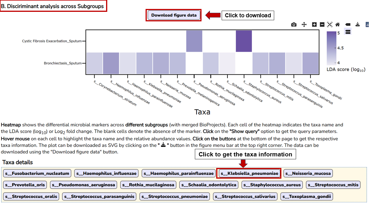
Merged BioProject wise
This heatmap shows microbial markers in the respective subgroups by merging the Bioprojects. Here, LEfSe method was chosen to find the differential markers. The blank cells indicate absence of the taxa. The colour intensity denotes the LDA score (log10). LDA score signifies the effect size of each differentially abundant microbe. Hover mouse on each cell to highlight the taxa name, subgroup, isolation source, BioProject and the LDA score. Click on "↓" button at the top right corner of the plot to download the plot in SVG format. Click on "Download figure data" button to download the data used to plot the figure. Click on the microbe buttons below the plot to view detailed information in the Taxa page.
Microbe Search
Users can search for specific microbial taxa (Genus or Species) of Domain Bacteria, Eukaryota (e.g. Fungi and Protozoa), Virus and Archaea with their scientific name as valid search term. For example, genus Aspergillus is shown here. Submitting the query will open a table of taxa with the name Aspergillus including the species as shown below. The result of the taxa search shows a list of microbes matching the query. Click on a specific taxon to view detailed information of the microbe in the Taxa page.
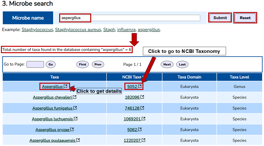
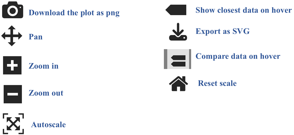
Figure buttons
Users can modify each figures in MDPD with the following buttons.
Disclaimer: This page is created using DokuWiki.